Fibonacci Heaps

This past Saturday, Westmont College hosted its annual Mathematics Field Day. This is a competition open to a few local high schoolers. This year, I could not attend the competition day because FemSTEM had our first community event. We had 30 girls from local elementary schools, Oaks Christian, and James Storehouse coming for our 6 different STEM station. So, because I could not compete in person at Westmont, I helped work on the Chalk Talk. Most of the work is also attributed to John Chung and Ethan Bergman who toiled with me to chose a interesting topic and make these slides. Similar to last year, the topic was “Fibonacci Numbers.“ We chose to focus on Fibonacci Heaps, a type of data structure. This presentation won the event (two years in a row!!), and I have added explanations to each slide at you continue through this post. I hope you enjoy!

The rest of the slides will generalize a data tree into one shows above. The image below then labels the landmarks of a data tree which will again be useful in the rest of the explanation.

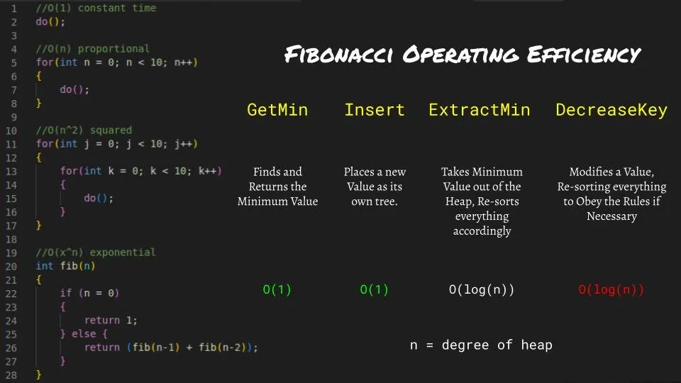
Operating efficiency is a way to measure the complexity and run time of a data structure. This uses O notation. Ideally, different commands (in the yellow text) would be able to run in O(1) time as it is constant. O(log n) time increases in time as the data tree grows in scale. This is what Fibonacci trees will try to better, specifically the Insert command and Decrease Key command. The video below shows how Fibonacci Trees are instead used to organize data and combine trees of like degree. It also details the rules and distinguishing factors between Fibonacci trees and binary trees which were shown above.

Using the Fibonacci Tree as a way to sort data on a large scale, the Insert command operating efficiency can be simplified to now take constant time, which is shown in the rest of this presentation.

Inserting a value into a tree requires the tree to sort all of the numbers before it to ensure that the correct order is maintained. We can calculate and simplify its operating efficiently using Amortized analysis, which is shown below.

When executing any commands, they normally run in sequence with each other. When inserting something, for example, there is also a sort command that must be executed that takes more time than inserting. We can attribute the time that it takes to sort() the data and distribute it over the rest of the add commands. This means that the actual sort command is now in constant time. The entire process still takes the same amount of time, but sort() now has less time attributed to its own run time. This is especially helpful in very large scale data sets when you don’t need to access the data often.

The previous two slides were a visualization of this amortized analysis and how time is distributed over a sorting command.

Notice how this amortized analysis decreased the insert time to become constant now.

Now we will talk about repeating a similar process for the DecreaseKey command. DecreaseKey is when a nodes value is changed and it is completely cut out of a data tree:

This is when the Fibonacci Sequence comes into use. Just like in nature, these Data trees grow logarithmically as well at the rate of the golden ratio, with the minimum of each tree increasing by the Fibonacci numbers! This is where these trees get the name!

I think it is really cool how just like in nature, data growth and sorting is maximized by the Fibonacci sequence as well. The complexity of each function is either bettered or not affected by using a Fibonacci Heap. Although I really don’t know that much about data science as a whole, I love this concept because of how mathematical it all is along with how similar it is to naturally occurring processes. Shoutout to Ethan Bergman and John Chung who presented the talk at the Westmont competition day and finalized this presentations first place!